Online Tutorials
Here we have provided several interesting online tutorials to help better use this open-source Python library PyPop7 for black-box optimization (BBO), as shown below:
Lens Shape Optimization from [Beyer, GECCO],
Lennard-Jones Cluster Optimization from pagmo (developed by European Space Agency),
Global Trajectory Optimization from pykep (developed by European Space Agency),
Benchmarking for Large-Scale Black-Box Optimization (LBO),
Controller Design/Optimization (aka Direct Policy Search),
Benchmarking BBO on the Well-Designed COCO Platform (A SIGEVO Impact Award for COCO),
Benchmarking BBO on the Famous NeverGrad Platform (Developed by FacebookResearch).
For each black-box optimizer from this open-source library, we have also provided a toy example on their corresponding API documentations and two testing code (if possible) on their corresponding Python source code folders.
Lens Shape Optimization
This figure shows an interesting evolution process of the lens shape, optimized by MAES, a simplified modern version of the well-established CMA-ES algorithm (nearly without significant performance loss). Its main objective is to find the optimal shape of glass body such that parallel incident light rays are concentrated in a given point on a plane while using a minimum of glass material possible. Refer to [Beyer, 2020, GECCO] for more mathematical details about this 15-dimensional objective function used here. To repeat this above figure, please run the following Python code:
# Written/Checked by Guochen Zhou, Minghan Zhang, Yajing Tan, and *Qiqi Duan*
import numpy as np
import imageio.v2 as imageio  # for animation
import matplotlib.pyplot as plt  # for static plotting
from matplotlib.path import Path  # for static plotting
import matplotlib.patches as patches  # for static plotting

from pypop7.optimizers.es.es import ES  # abstract class for all evolution Strategies
from pypop7.optimizers.es.maes import MAES  # Matrix Adaptation Evolution Strategy


# <1> - Set Parameters for Lens Shape Optimization
weight = 0.9  # weight of focus function
r = 7  # radius of lens
h = 1  # trapezoidal slices of height
b = 20  # distance between lens and object
eps = 1.5  # refraction index
d_init = 3  # initialization


# <2> - Define Objective Function (aka Fitness Function) to be *Minimized*
def func_lens(x):  # refer to [Beyer, 2020, ACM-GECCO] for all mathematical details
    n = len(x)
    focus = r - ((h*np.arange(1, n) - 0.5) + b/h*(eps - 1)*np.transpose(np.abs(x[1:]) - np.abs(x[:(n-1)])))
    mass = h*(np.sum(np.abs(x[1:(n-1)])) + 0.5*(np.abs(x[0]) + np.abs(x[n-1])))
    return weight*np.sum(focus**2) + (1.0 - weight)*mass


def get_path(x):  # only for plotting
    left, right, height = [], [], r
    for i in range(len(x)):
        x[i] = -x[i] if x[i] < 0 else x[i]
        left.append((-0.5*x[i], height))
        right.append((0.5*x[i], height))
        height -= 1
    points = left
    for i in range(len(right)):
        points.append(right[-i - 1])
    points.append(left[0])
    codes = [Path.MOVETO]
    for i in range(len(points) - 2):
        codes.append(Path.LINETO)
    codes.append(Path.CLOSEPOLY)
    return Path(points, codes)


def plot(xs):
    file_names, frames = [], []
    for i in range(len(xs)):
        sub_figure = '_' + str(i) + '.png'
        fig = plt.figure()
        ax = fig.add_subplot(111)
        plt.rcParams['font.family'] = 'Times New Roman'
        plt.rcParams['font.size'] = '12'
        ax.set_xlim(-10, 10)
        ax.set_ylim(-8, 8)
        path = get_path(xs[i])
        patch = patches.PathPatch(path, facecolor='orange', lw=2)
        ax.add_patch(patch)
        plt.savefig(sub_figure)
        file_names.append(sub_figure)
    for image in file_names:
        frames.append(imageio.imread(image))
    imageio.mimsave('lens_shape_optimization.gif', frames, 'GIF', duration=0.3)


# <3> - Extend Optimizer Class MAES to Generate Data for Plotting
class MAESPLOT(MAES):  # to overwrite original MAES algorithm for plotting
    def optimize(self, fitness_function=None, args=None):  # for all generations (iterations)
        fitness = ES.optimize(self, fitness_function)
        z, d, mean, s, tm, y = self.initialize()
        xs = [mean.copy()]  # for plotting
        while not self._check_terminations():
            z, d, y = self.iterate(z, d, mean, tm, y, args)
            if self.saving_fitness and (not self._n_generations % self.saving_fitness):
                xs.append(self.best_so_far_x)  # for plotting
            mean, s, tm = self._update_distribution(z, d, mean, s, tm, y)
            self._print_verbose_info(fitness, y)
            self._n_generations += 1
            if self.is_restart:
                z, d, mean, s, tm, y = self.restart_reinitialize(z, d, mean, s, tm, y)
        res = self._collect(fitness, y, mean)
        res['xs'] = xs  # for plotting
        return res


if __name__ == '__main__':
    ndim_problem = 15  # dimension of objective function
    problem = {'fitness_function': func_lens,  # objective (fitness) function
               'ndim_problem': ndim_problem,  # number of dimensionality of objective function
               'lower_boundary': -5.0*np.ones((ndim_problem,)),  # lower boundary of search range
               'upper_boundary': 5.0*np.ones((ndim_problem,))}  # upper boundary of search range
    options = {'max_function_evaluations': 7e3,  # maximum of function evaluations
               'seed_rng': 2022,  # seed of random number generation (for repeatability)
               'x': d_init*np.ones((ndim_problem,)),  # initial mean of Gaussian search distribution
               'sigma': 0.3,  # global step-size of Gaussian search distribution (not necessarily an optimal value)
               'saving_fitness': 50,  # to record best-so-far fitness every 50 function evaluations
               'is_restart': False}  # whether or not to run the (default) restart process
    results = MAESPLOT(problem, options).optimize()
    plot(results['xs'])
As written by Darwin, “If it could be demonstrated that any complex organ existed, which could not possibly have been formed by numerous, successive, slight modifications, my theory would absolutely break down.” Luckily, the evolution of an eye-lens could indeed proceed through many small steps from only the optimization (rather biological) view of point.
For more interesting applications of ES / CMA-ES / NES on many challenging optimization problems, refer to e.g., [Lee et al., 2023, Science Robotics]; [Sun et al., 2023, ACL]; [Koginov et al., 2023, IEEE-TMRB]; [Lange et al., 2023, ICLR]; [Yu et al., 2023, IJCAI]; [Kim et al., 2023, Science Robotics]; [Slade et al., 2022, Nature]; [De Croon et al., 2022, Nature]; [Sun et al., 2022, ICML]; [Wang&Ponce, 2022, GECCO]; [Bharti et al., 2022, Rev. Mod. Phys]; [Nomura et al., 2021, AAAI], [Anand et al., 2021, Mach. Learn.: Sci. Technol.], [Maheswaranathan et al., 2019, ICML], [Dong et al., 2019, CVPR]; [Ha&Schmidhuber, 2018, NeurIPS]; [OpenAI, 2017], [Zhang et al., 2017, Science], [Agrawal et al., 2014, TVCG], [Koumoutsakos et al., 2001, AIAA], [Lipson&Pollack, 2000, Nature], just to name a few. For a systematical paper collection on some top-tier journals/conferences, please refer to https://github.com/Evolutionary-Intelligence/DistributedEvolutionaryComputation.
Lennard-Jones Cluster Optimization
Note that the above figure (i.e., three clusters of atoms) is taken directly from Prof. Jonathan Doye of Oxford University. In chemistry, Lennard-Jones Cluster Optimization is a popular single-objective real-parameter (black-box) optimization problem, which is to minimize the energy of a cluster of atoms assuming a Lennard-Jones potential between each pair. Here, we use two different Differential Evolution (DE) versions to solve this high-dimensional optimization problem:
import pygmo as pg  # need to be installed: https://esa.github.io/pygmo2/install.html
import seaborn as sns
import matplotlib.pyplot as plt

from pypop7.optimizers.de.cde import CDE  # https://pypop.readthedocs.io/en/latest/de/cde.html
from pypop7.optimizers.de.jade import JADE  # https://pypop.readthedocs.io/en/latest/de/jade.html


# see https://esa.github.io/pagmo2/docs/cpp/problems/lennard_jones.html for the fitness function
prob = pg.problem(pg.lennard_jones(150))
print(prob)  # 444-dimensional


def energy_func(x):  # wrapper to obtain fitness of type `float`
    return float(prob.fitness(x))


if __name__ == '__main__':
    results = []  # to save all optimization results from different optimizers
    for DE in [CDE, JADE]:
        problem = {'fitness_function': energy_func,
                   'ndim_problem': 444,
                   'upper_boundary': prob.get_bounds()[1],
                   'lower_boundary': prob.get_bounds()[0]}
        if DE == JADE:  # for JADE (but not for CDE)
            is_bound = True
        else:
            is_bound = False
        options = {'max_function_evaluations': 400000,
                   'seed_rng': 2022,  # for repeatability
                   'saving_fitness': 1,  # to save all fitness generated during optimization
                   'is_bound': is_bound}
        solver = DE(problem, options)
        results.append(solver.optimize())
        print(results[-1])

    sns.set_theme(style='darkgrid')
    plt.figure()
    for label, res in zip(['CDE', 'JADE'], results):
        plt.plot(res['fitness'][250000:, 0], res['fitness'][250000:, 1], label=label)

    plt.legend()
    plt.show()
The two convergence curves generated for CDE (without box constraints) and JADE (with box constraints) are presented in the following image (starting from 250000-th generations can avoid excessively high fitness values generated during the early stage to disrupt convergence curves):
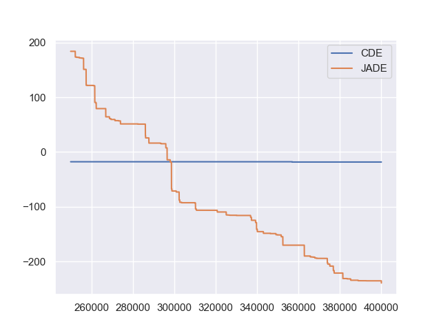
From the above figure, two different DE versions show different search performance: CDE does not limit samples into the given search boundaries during optimization and generate a out-of-box solution (which may be infeasible in practice) very fast, while JADE limits all samples into the given search boundaries during optimization and generate an inside-of-box solution relatively slow. Since different implementations of the same algorithm family could sometimes even result in totally different search behaviors, their open-source implementations play an important role for repeatability.
For more interesting applications of DE on challenging problems, refer to e.g., [Higgins et al., 2023, Science]; [McNulty et al., 2023, PRL]; [An et al., 2020, PNAS]; [Gagnon et al., 2017, PRL]; [Laganowsky et al., 2014, Nature]; [Lovett et al., 2013, PRL], just to name a few. For a systematical paper collection of evolutionary algorithms on some top-tier journals/conferences, please refer to https://github.com/Evolutionary-Intelligence/DistributedEvolutionaryComputation.
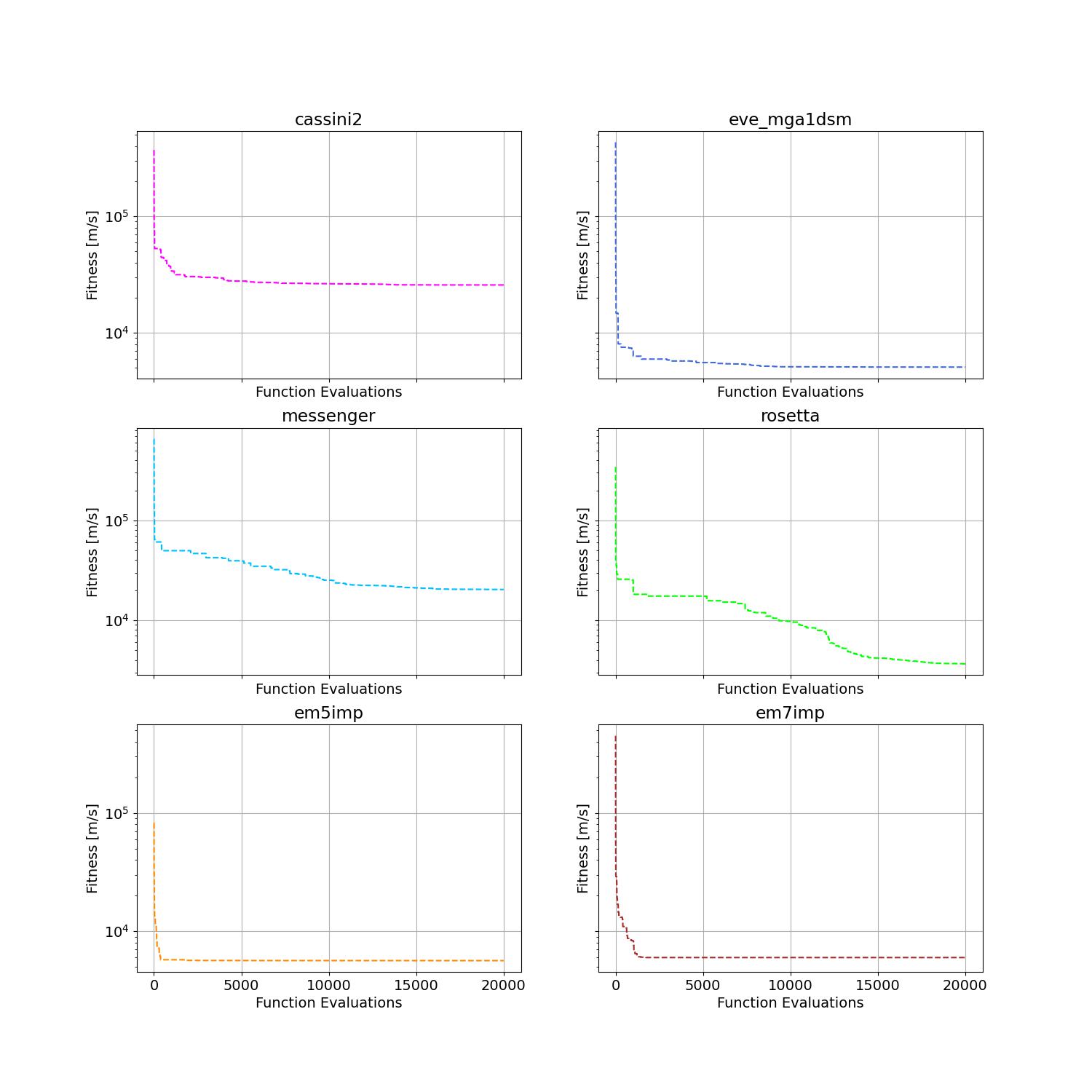
Global Trajectory Optimization from PyKep
Six hard global trajectory optimization (GTO) problems have been given in pykep, developed at European Space Agency. Here we use the Standard Particle Swarm Optimizer (SPSO) as a black-box optimizer baseline:
"""Demo that uses PSO to optimize 6 GTO problems provided by `pykep`:
    https://esa.github.io/pykep/
    https://esa.github.io/pykep/examples/ex13.html
"""
import pygmo as pg  # it's better to use conda to install (and it's better to use pygmo==2.18)
import pykep as pk  # it's better to use conda to install
import matplotlib.pyplot as plt

from pypop7.optimizers.pso.spso import SPSO as Solver


fig, axes = plt.subplots(nrows=3, ncols=2, sharex='col', sharey='row', figsize=(15, 15))
problems = [pk.trajopt.gym.cassini2, pk.trajopt.gym.eve_mga1dsm, pk.trajopt.gym.messenger,
            pk.trajopt.gym.rosetta, pk.trajopt.gym.em5imp, pk.trajopt.gym.em7imp]
ticks = [0, 5e3, 1e4, 1.5e4, 2e4]

for prob_number in range(0, 6):
    udp = problems[prob_number]

    def fitness_func(x):  # wrapper of fitness function
        return udp.fitness(x)[0]

    prob = pg.problem(udp)
    print(prob)
    pro = {'fitness_function': fitness_func,
           'ndim_problem': prob.get_nx(),
           'lower_boundary': prob.get_lb(),
           'upper_boundary': prob.get_ub()}
    opt = {'seed_rng': 0,
           'max_function_evaluations': 2e4,
           'saving_fitness': 1,
           'is_bound': True}
    solver = Solver(pro, opt)
    res = solver.optimize()
    if prob_number == 0:
        axes[0, 0].semilogy(res['fitness'][:, 0], res['fitness'][:, 1], '--', color='fuchsia', label='SPSO')
        axes[0, 0].set_title('cassini2')
    elif prob_number == 1:
        axes[0, 1].semilogy(res['fitness'][:, 0], res['fitness'][:, 1], '--', color='royalblue', label='SPSO')
        axes[0, 1].set_title('eve_mga1dsm')
    elif prob_number == 2:
        axes[1, 0].semilogy(res['fitness'][:, 0], res['fitness'][:, 1], '--', color='deepskyblue', label='SPSO')
        axes[1, 0].set_title('messenger')
    elif prob_number == 3:
        axes[1, 1].semilogy(res['fitness'][:, 0], res['fitness'][:, 1], '--', color='lime', label='SPSO')
        axes[1, 1].set_title('rosetta')
    elif prob_number == 4:
        axes[2, 0].semilogy(res['fitness'][:, 0], res['fitness'][:, 1], '--', color='darkorange', label='SPSO')
        axes[2, 0].set_title('em5imp')
    elif prob_number == 5:
        axes[2, 1].semilogy(res['fitness'][:, 0], res['fitness'][:, 1], '--', color='brown', label='SPSO')
        axes[2, 1].set_title('em7imp')
for ax in axes.flat:
    ax.set(xlabel='Function Evaluations', ylabel='Fitness [m/s]')
    ax.set_xticks(ticks)
    ax.grid()
plt.savefig('pykep_optimization.jpg')  # to save locally
The convergence curves on six different instances obtained via SPSO are given below:
For more applications of PSO on some challenging problems, refer to e.g., [Reddy et al., 2023, TC]; [Guan et al., 2022, PRL]; [Weiel, et al., 2021, Nature Mach. Intell.]; [Tang et al., 2019, TPAMI]; [ Villeneuve et al., 2017, Science]; [Zhang et al., 2015, IJCV]; [Sharp et al., 2015, CHI]; [Tompson et al., 2014, TOG]; [Baca et al., 2013, Cell]; [Kim et al., 2012, Nature]; just to name a few. For a systematical paper collection on some top-tier journals/conferences, please refer to https://github.com/Evolutionary-Intelligence/DistributedEvolutionaryComputation.
Benchmarking for Large-Scale Black-Box Optimization (LBO)
Benchmarking of BBO algorithms plays a very crucial role on understanding their search dynamics, comparing their competitive performance, analyzing their advantages/limitations, and also choosing their state-of-the-art (SOTA) versions, usually before applying them to challenging real-world problems.
Note
“A biased benchmark, excluding large parts of the real-world needs, leads to biased conclusions, no matter how many experiments we perform.” —[Meunier et al., 2022, TEVC]
Here we show how to benchmark multiple black-box optimizers on a relatively large collection of test functions for LBO, in order to mainly compare their local search capabilities:
First, as a standard benchmarking practice, generate shift vectors and rotation matrices needed in the experiments, which is used to avoid possible bias against center and separability:
import time

import numpy as np

from pypop7.benchmarks.shifted_functions import generate_shift_vector
from pypop7.benchmarks.rotated_functions import generate_rotation_matrix


def generate_sv_and_rm(functions=None, ndims=None, seed=None):
    if functions is None:
        functions = ['sphere', 'cigar', 'discus', 'cigar_discus', 'ellipsoid',
                     'different_powers', 'schwefel221', 'step', 'rosenbrock', 'schwefel12']
    if ndims is None:
        ndims = [2, 10, 100, 200, 1000, 2000]
    if seed is None:
        seed = 20221001

    rng = np.random.default_rng(seed)
    seeds = rng.integers(np.iinfo(np.int64).max, size=(len(functions), len(ndims)))

    for i, f in enumerate(functions):
        for j, d in enumerate(ndims):
            generate_shift_vector(f, d, -9.5, 9.5, seeds[i, j])

    start_run = time.time()
    for i, f in enumerate(functions):
        for j, d in enumerate(ndims):
            start_time = time.time()
            generate_rotation_matrix(f, d, seeds[i, j])
            print('* {:d}-d {:s}: runtime {:7.5e}'.format(
                d, f, time.time() - start_time))
    print('*** Total runtime: {:7.5e}.'.format(time.time() - start_run))


if __name__ == '__main__':
    generate_sv_and_rm()
Then, invoke multiple black-box optimizers from PyPop7 on these (rotated and shifted) test functions:
import os
import time
import pickle
import argparse

import numpy as np

import pypop7.benchmarks.continuous_functions as cf


class Experiment(object):
    def __init__(self, index, function, seed, ndim_problem):
        self.index, self.seed = index, seed
        self.function, self.ndim_problem = function, ndim_problem
        # save all data generated during optimization
        self._folder = 'pypop7_benchmarks_lso'
        if not os.path.exists(self._folder):
            os.makedirs(self._folder)
        # set file format
        self._file = os.path.join(self._folder, 'Algo-{}_Func-{}_Dim-{}_Exp-{}.pickle')

    def run(self, optimizer):
        problem = {'fitness_function': self.function,
                   'ndim_problem': self.ndim_problem,
                   'upper_boundary': 10.0 * np.ones((self.ndim_problem,)),
                   'lower_boundary': -10.0 * np.ones((self.ndim_problem,))}
        options = {'max_function_evaluations': 100000 * self.ndim_problem,
                   'max_runtime': 3600 * 3,  # seconds (=3 hours)
                   'fitness_threshold': 1e-10,
                   'seed_rng': self.seed,
                   'sigma': 20.0 / 3.0,
                   'saving_fitness': 2000,
                   'verbose': 0}
        options['temperature'] = 100.0  # for simulated annealing (SA)
        solver = optimizer(problem, options)
        results = solver.optimize()
        file = self._file.format(solver.__class__.__name__,
                                 solver.fitness_function.__name__,
                                 solver.ndim_problem,
                                 self.index)
        with open(file, 'wb') as handle:  # data format (pickle)
            pickle.dump(results, handle, protocol=pickle.HIGHEST_PROTOCOL)


class Experiments(object):
    def __init__(self, start, end, ndim_problem):
        self.start, self.end = start, end
        self.ndim_problem = ndim_problem
        self.functions = [cf.sphere, cf.cigar,
                          cf.discus, cf.cigar_discus,
                          cf.ellipsoid, cf.different_powers,
                          cf.schwefel221, cf.step,
                          cf.rosenbrock, cf.schwefel12]
        # set RNG seeds for repeatability
        self.seeds = np.random.default_rng(2022).integers(
            np.iinfo(np.int64).max, size=(len(self.functions), 50))

    def run(self, optimizer):
        for index in range(self.start, self.end + 1):
            print('* experiment: {:d} ***:'.format(index))
            for i, f in enumerate(self.functions):
                start_time = time.time()
                print('  * function: {:s}:'.format(f.__name__))
                experiment = Experiment(index, f, self.seeds[i, index], self.ndim_problem)
                experiment.run(optimizer)
                print('    runtime: {:7.5e}.'.format(time.time() - start_time))


if __name__ == '__main__':
    start_runtime = time.time()
    parser = argparse.ArgumentParser()
    # set starting index of experiments (from 0 to 49)
    parser.add_argument('--start', '-s', type=int)
    # set ending index of experiments (from 0 to 49)
    parser.add_argument('--end', '-e', type=int)
    # use any optimizer from PyPop7
    parser.add_argument('--optimizer', '-o', type=str)
    # set dimension of all fitness functions
    parser.add_argument('--ndim_problem', '-d', type=int, default=2000)
    args = parser.parse_args()
    params = vars(args)
    # ensure seeds between 0 (include) and 49 (include)
    assert isinstance(params['start'], int) and 0 <= params['start'] < 50
    assert isinstance(params['end'], int) and 0 <= params['end'] < 50
    assert isinstance(params['optimizer'], str)
    assert isinstance(params['ndim_problem'], int) and params['ndim_problem'] > 0
    if params['optimizer'] == 'PRS':  # 1952
        # PRS: Ashby's "Design for a Brain: The Origin of Adaptive Behavior"
        #   (1952 - 1st Edition / 1960 - 2nd Edition)
        #   https://link.springer.com/book/10.1007/978-94-015-1320-3
        from pypop7.optimizers.rs.prs import PRS as Optimizer
    elif params['optimizer'] == 'SRS':  # 2001
        from pypop7.optimizers.rs.srs import SRS as Optimizer
    elif params['optimizer'] == 'ARHC':  # 2008
        from pypop7.optimizers.rs.arhc import ARHC as Optimizer
    elif params['optimizer'] == 'GS':  # 2017
        from pypop7.optimizers.rs.gs import GS as Optimizer
    elif params['optimizer'] == 'BES':
        from pypop7.optimizers.rs.bes import BES as Optimizer
    elif params['optimizer'] == 'HJ':
        from pypop7.optimizers.ds.hj import HJ as Optimizer
    elif params['optimizer'] == 'NM':
        from pypop7.optimizers.ds.nm import NM as Optimizer
    elif params['optimizer'] == 'POWELL':
        from pypop7.optimizers.ds.powell import POWELL as Optimizer
    elif params['optimizer'] == 'FEP':
        from pypop7.optimizers.ep.fep import FEP as Optimizer
    elif params['optimizer'] == 'GENITOR':
        from pypop7.optimizers.ga.genitor import GENITOR as Optimizer
    elif params['optimizer'] == 'G3PCX':
        from pypop7.optimizers.ga.g3pcx import G3PCX as Optimizer
    elif params['optimizer'] == 'GL25':
        from pypop7.optimizers.ga.gl25 import GL25 as Optimizer
    elif params['optimizer'] == 'COCMA':
        from pypop7.optimizers.cc.cocma import COCMA as Optimizer
    elif params['optimizer'] == 'HCC':
        from pypop7.optimizers.cc.hcc import HCC as Optimizer
    elif params['optimizer'] == 'SPSO':
        from pypop7.optimizers.pso.spso import SPSO as Optimizer
    elif params['optimizer'] == 'SPSOL':
        from pypop7.optimizers.pso.spsol import SPSOL as Optimizer
    elif params['optimizer'] == 'CLPSO':
        from pypop7.optimizers.pso.clpso import CLPSO as Optimizer
    elif params['optimizer'] == 'CCPSO2':
        from pypop7.optimizers.pso.ccpso2 import CCPSO2 as Optimizer
    elif params['optimizer'] == 'CDE':
        from pypop7.optimizers.de.cde import CDE as Optimizer
    elif params['optimizer'] == 'JADE':
        from pypop7.optimizers.de.jade import JADE as Optimizer
    elif params['optimizer'] == 'SHADE':
        from pypop7.optimizers.de.shade import SHADE as Optimizer
    elif params['optimizer'] == 'SCEM':
        from pypop7.optimizers.cem.scem import SCEM as Optimizer
    elif params['optimizer'] == 'MRAS':
        from pypop7.optimizers.cem.mras import MRAS as Optimizer
    elif params['optimizer'] == 'DSCEM':
        from pypop7.optimizers.cem.dscem import DSCEM as Optimizer
    elif params['optimizer'] == 'UMDA':
        from pypop7.optimizers.eda.umda import UMDA as Optimizer
    elif params['optimizer'] == 'EMNA':
        from pypop7.optimizers.eda.emna import EMNA as Optimizer
    elif params['optimizer'] == 'RPEDA':
        from pypop7.optimizers.eda.rpeda import RPEDA as Optimizer
    elif params['optimizer'] == 'XNES':
        from pypop7.optimizers.nes.xnes import XNES as Optimizer
    elif params['optimizer'] == 'SNES':
        from pypop7.optimizers.nes.snes import SNES as Optimizer
    elif params['optimizer'] == 'R1NES':
        from pypop7.optimizers.nes.r1nes import R1NES as Optimizer
    elif params['optimizer'] == 'CMAES':
        from pypop7.optimizers.es.cmaes import CMAES as Optimizer
    elif params['optimizer'] == 'FMAES':
        from pypop7.optimizers.es.fmaes import FMAES as Optimizer
    elif params['optimizer'] == 'RMES':
        from pypop7.optimizers.es.rmes import RMES as Optimizer
    elif params['optimizer'] == 'VDCMA':
        from pypop7.optimizers.es.vdcma import VDCMA as Optimizer
    elif params['optimizer'] == 'LMMAES':
        from pypop7.optimizers.es.lmmaes import LMMAES as Optimizer
    elif params['optimizer'] == 'MMES':
        from pypop7.optimizers.es.mmes import MMES as Optimizer
    elif params['optimizer'] == 'LMCMA':
        from pypop7.optimizers.es.lmcma import LMCMA as Optimizer
    elif params['optimizer'] == 'LAMCTS':
        from pypop7.optimizers.bo.lamcts import LAMCTS as Optimizer
    else:
        raise ValueError(f"Cannot find optimizer class {params['optimizer']} in PyPop7!")
    experiments = Experiments(params['start'], params['end'], params['ndim_problem'])
    experiments.run(Optimizer)
    print('Total runtime: {:7.5e}.'.format(time.time() - start_runtime))
Please run the above Python script (named as run_experiments.py here) in the background on a high-performing computing server, since typically it needs a very long runtime for LBO:
$ # on Linux
$ nohup python run_experiments.py -s=1 -e=2 -o=LMCMA >LMCMA_1_2.out 2>&1 &
To further compare global search capabilities of different black-box optimizers for LBO, please use the benchmarking test suite: benchmark_global_search().
Controller Design/Optimization
Using population-based (e.g., evolutionary) optimization methods to design robot controllers has a relatively long history. Recently, the increasing availability of distributed computing makes them a competitive alternative to RL, as empirically demonstrated in OpenAI’s 2017 research report. Here, we provide a very simplified demo to show how ES works well on a classical control problem called CartPole:
"""This is a simple demo to optimize a linear controller
   on the popular `gymnasium` platform for RL:
    https://github.com/Farama-Foundation/Gymnasium

    $ pip install gymnasium
    $ pip install gymnasium[classic-control]

    For benchmarking, please use more challenging MuJoCo tasks:
    https://mujoco.org/
"""
import numpy as np
# to be installed from https://github.com/Farama-Foundation/Gymnasium
import gymnasium as gym

from pypop7.optimizers.es.maes import MAES as Solver


class Controller:  # linear controller for simplicity
    def __init__(self):
        self.env = gym.make('CartPole-v1', render_mode='human')
        self.observation, _ = self.env.reset()
        # for action probability space
        self.action_dim = self.env.action_space.n

    def __call__(self, x):
        rewards = 0
        self.observation, _ = self.env.reset()
        for i in range(1000):
            action = np.matmul(x.reshape(self.action_dim, -1), self.observation[:, np.newaxis])
            actions = np.sum(action)
            prob_left, prob_right = action[0]/actions, action[1]/actions  # seen as a probability
            action = 1 if prob_left < prob_right else 0
            self.observation, reward, terminated, truncated, _ = self.env.step(action)
            rewards += reward
            if terminated or truncated:
                return -rewards  # for minimization (rather than maximization)
        return -rewards  # to negate rewards


if __name__ == '__main__':
    c = Controller()
    pro = {'fitness_function': c,
           'ndim_problem': len(c.observation)*c.action_dim,
           'lower_boundary': -10*np.ones((len(c.observation)*c.action_dim,)),
           'upper_boundary': 10*np.ones((len(c.observation)*c.action_dim,))}
    opt = {'max_function_evaluations': 1e4,
           'seed_rng': 0,
           'sigma': 3.0,
           'verbose': 1}
    solver = Solver(pro, opt)
    print(solver.optimize())
    c.env.close()
Benchmarking BBO on the Well-Designed COCO Platform
From the evolutionary computation community, COCO is a well-designed and actively-maintained software platform for comparing continuous optimizers in the black-box setting.
"""Demo for `COCO` benchmarking using only `PyPop7` here:
   https://github.com/numbbo/coco

   To install `COCO` successfully, please read the above open link carefully.
"""
import os
import webbrowser  # for post-processing in the browser

import numpy as np
import cocoex  # experimentation module of `COCO`
import cocopp  # post-processing module of `COCO`

from pypop7.optimizers.es.maes import MAES


if __name__ == '__main__':
    suite, output = 'bbob', 'COCO-PyPop7-MAES'
    budget_multiplier = 1e3  # or 1e4, 1e5, ...
    observer = cocoex.Observer(suite, 'result_folder: ' + output)
    minimal_print = cocoex.utilities.MiniPrint()
    for function in cocoex.Suite(suite, '', ''):
        function.observe_with(observer)  # to generate data for `cocopp` post-processing
        sigma = np.min(function.upper_bounds - function.lower_bounds) / 3.0
        problem = {'fitness_function': function,
                   'ndim_problem': function.dimension,
                   'lower_boundary': function.lower_bounds,
                   'upper_boundary': function.upper_bounds}
        options = {'max_function_evaluations': function.dimension * budget_multiplier,
                   'seed_rng': 2022,
                   'x': function.initial_solution,
                   'sigma': sigma}
        solver = MAES(problem, options)
        print(solver.optimize())
    cocopp.main(observer.result_folder)
    webbrowser.open('file://' + os.getcwd() + '/ppdata/index.html')
The final output of the above code looks like:


Benchmarking BBO on the Famous NeverGrad Platform
As pointed out in the recent paper from Facebook AI Research ([Meunier et al., 2022, TEVC]), “Existing studies in black-box optimization suffer from low generalizability, caused by a typically selective choice of problem instances used for training and testing of different optimization algorithms. Among other issues, this practice promotes overfitting and poor-performing user guidelines.”
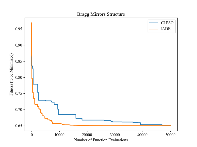
Here we choose a real-world optimization problem to compare two population-based optimizers (PSO vs DE) in the following:
"""Demo that optimizes the Bragg mirrors structure, modeled in the following paper:
    Bennet, P., Centeno, E., Rapin, J., Teytaud, O. and Moreau, A., 2020.
    The photonics and ARCoating testbeds in NeverGrad.
    https://hal.uca.fr/hal-02613161v1
"""
import numpy as np
import matplotlib.pyplot as plt
from nevergrad.functions.photonics.core import Photonics

from pypop7.optimizers.pso.clpso import CLPSO  # https://pypop.readthedocs.io/en/latest/pso/clpso.html
from pypop7.optimizers.de.jade import JADE  # https://pypop.readthedocs.io/en/latest/de/jade.html


if __name__ == '__main__':
    plt.figure(figsize=(8, 6))
    plt.rcParams['font.family'] = 'Times New Roman'
    plt.rcParams['font.size'] = '12'

    labels = ['CLPSO', 'JADE']
    for i, Opt in enumerate([CLPSO, JADE]):
        ndim_problem = 10  # dimension of objective function
        half = int(ndim_problem/2)
        func = Photonics("bragg", ndim_problem)
        problem = {'fitness_function': func,
                   'ndim_problem': ndim_problem,
                   'lower_boundary': np.hstack((2*np.ones(half), 30*np.ones(half))),
                   'upper_boundary': np.hstack((3*np.ones(half), 180*np.ones(half)))}
        options = {'max_function_evaluations': 50000,
                   'n_individuals': 200,
                   'is_bound': True,
                   'seed_rng': 0,
                   'saving_fitness': 1,
                   'verbose': 200}
        solver = Opt(problem, options)
        results = solver.optimize()
        res = results['fitness']
        plt.plot(res[:, 0], res[:, 1], linewidth=2.0, linestyle='-', label=labels[i])
    plt.legend()
    plt.xlabel('Number of Function Evaluations')
    plt.ylabel('Fitness (to be Minimized)')
    plt.title('Bragg Mirrors Structure')
    plt.savefig('photonics_optimization.png')
The final figure output is shown below:
More Usage Examples
For each black-box optimizer from this open-source Python library, we have also provide a toy example on their corresponding API documentations and two testing code (if possible) on their corresponding source code folders. For a summary of its applications and praises (from others), please refer to this html.