User Guide

Before applying pypop7 to real-world black-box optimization (BBO) problems, the following user guidelines should be read: problem definition, optimizer setting, result analysis, and algorithm selection and configuration.

Problem Definition

First, an objective function (called fitness function in this library) needs to be defined in the function form. Then, the standard data structure dict is used as a simple yet effective way to store all settings related to the optimization problem at hand, such as:

• fitness_function: objective function to be minimized (func),

• ndim_problem: number of dimensionality (int),

• upper_boundary: upper boundary of search range (array_like),

• lower_boundary: lower boundary of search range (array_like).

Note that without loss of generality, only the minimization process is considered in this library, since maximization can be easily transferred to minimization by negating it.

Below is a simple example to define the well-known test function Rosenbrock:

>>> import numpy as np
>>> def rosenbrock(x):  # define the fitness (cost/objective) function
...     return 100.0*np.sum(np.power(x[1:] - np.power(x[:-1], 2), 2)) + np.sum(np.power(x[:-1] - 1, 2))
>>> ndim_problem = 1000  # define its settings
>>> problem = {'fitness_function': rosenbrock,  # cost function
...            'ndim_problem': ndim_problem,  # dimension
...            'lower_boundary': -10.0*np.ones((ndim_problem,)),  # search boundary
...            'upper_boundary': 10.0*np.ones((ndim_problem,))}

When the fitness function itself involves other input arguments except the sampling point x (here we distinguish input arguments and above problem settings), there are two simple ways to support this scenario:

• to create a class wrapper, e.g.:

  >>> import numpy as np
  >>> def rosenbrock(x, arg):  # define the fitness (cost/objective) function
  ...     return arg*np.sum(np.power(x[1:] - np.power(x[:-1], 2), 2)) + np.sum(np.power(x[:-1] - 1, 2))
  >>> class Rosenbrock(object):  # build a class wrapper
  ...     def __init__(self, arg):  # arg is an extra input argument
  ...         self.arg = arg
  ...     def __call__(self, x):  # for fitness evaluation
  ...         return rosenbrock(x, self.arg)
  >>> rosen = Rosenbrock(100.0)
  >>> ndim_problem = 1000  # define its settings
  >>> problem = {'fitness_function': rosen,  # cost function
  ...            'ndim_problem': ndim_problem,  # dimension
  ...            'lower_boundary': -10.0*np.ones((ndim_problem,)),  # search boundary
  ...            'upper_boundary': 10.0*np.ones((ndim_problem,))}
  

• to utilize the easy-to-use unified interface provided for all optimizers in this library, e.g.:

  >>> import numpy as np
  >>> def rosenbrock(x, args):
  ...     return args*np.sum(np.power(x[1:] - np.power(x[:-1], 2), 2)) + np.sum(np.power(x[:-1] - 1, 2))
  >>> ndim_problem = 10
  >>> problem = {'fitness_function': rosenbrock,
  ...            'ndim_problem': ndim_problem,
  ...            'lower_boundary': -5*np.ones((ndim_problem,)),
  ...            'upper_boundary': 5*np.ones((ndim_problem,))}
  >>> from pypop7.optimizers.es.maes import MAES  # which can be replaced by any other optimizer in this library
  >>> options = {'fitness_threshold': 1e-10,  # terminate when the best-so-far fitness is lower than 1e-10
  ...            'max_function_evaluations': ndim_problem*10000,  # maximum of function evaluations
  ...            'seed_rng': 0,  # seed of random number generation (which must be set for repeatability)
  ...            'sigma': 3.0,  # initial global step-size of Gaussian search distribution
  ...            'verbose': 500}  # to print verbose information every 500 generations
  >>> maes = MAES(problem, options)  # initialize the optimizer
  >>> results = maes.optimize(args=100.0)  # args as input arguments of fitness function except sampling point
  >>> print(results['best_so_far_y'], results['n_function_evaluations'])
  3.98657911234714 100000  # this is a well-recognized *local* attractor rather than the global optimum
  

When there are multiple (>=2) input arguments except the sampling point x, all of them should be organized via a function or class wrapper with only one input argument except the sampling point x (in dict or tuple form).

Typically, upper_boundary and lower_boundary are enough for end-users to control the search range. However, sometimes for benchmarking-of-optimizers purpose (e.g., to avoid utilizing symmetry and origin to possibly bias the search), we add two extra settings to control the initialization of the population/individual:

• initial_upper_boundary: upper boundary only for initialization (array_like),

• initial_lower_boundary: lower boundary only for initialization (array_like).

if not given, both initial_upper_boundary and initial_lower_boundary are set to upper_boundary and lower_boundary, respectively. When initial_upper_boundary and initial_lower_boundary are explicitly given, the initialization of population/individual will be sampled from [initial_lower_boundary, initial_upper_boundary] rather than [lower_boundary, upper_boundary].

Optimizer Setting

This library provides a unified API for hyper-parameter settings of all black-box optimizers. The following algorithm options (all stored into a dict) are common for all optimizers:

• max_function_evaluations: maximum of function evaluations (int, default: np.Inf),

• max_runtime: maximal runtime to be allowed (float, default: np.Inf),

• seed_rng: seed for random number generation needed to be explicitly set (int).

At least one of two options (max_function_evaluations and max_runtime) should be set, according to the available computing resources or acceptable runtime.

For repeatability, seed_rng should be explicitly set for random number generation (RNG).

Note that for any optimizer, its specific options/settings (see its API documentation for details) can be naturally added into the dict data structure. Take the well-known Cross-Entropy Method (CEM) as an illustrative example. The settings of mean and std of its Gaussian sampling distribution usually have a significant impact on the convergence rate (see its API for more details about its hyper-parameters):

>>> import numpy as np
>>> from pypop7.benchmarks.base_functions import rosenbrock  # function to be minimized
>>> from pypop7.optimizers.cem.scem import SCEM
>>> problem = {'fitness_function': rosenbrock,  # define problem arguments
...            'ndim_problem': 10,
...            'lower_boundary': -5*np.ones((10,)),
...            'upper_boundary': 5*np.ones((10,))}
>>> options = {'max_function_evaluations': 1000000,  # set optimizer options
...            'seed_rng': 2022,
...            'mean': 4*np.ones((10,)),  # initial mean of Gaussian search distribution
...            'sigma': 3.0}  # initial std (aka global step-size) of Gaussian search distribution
>>> scem = SCEM(problem, options)  # initialize the optimizer class
>>> results = scem.optimize()  # run the optimization process
>>> # return the number of function evaluations and best-so-far fitness
>>> print(f"SCEM: {results['n_function_evaluations']}, {results['best_so_far_y']}")
SCEM: 1000000, 10.328016143160333

Result Analysis

After the ending of optimization stage, all optimizers return at least the following common results (collected into a dict) in a unified way:

• best_so_far_x: the best-so-far solution found during optimization,

• best_so_far_y: the best-so-far fitness (aka objective value) found during optimization,

• n_function_evaluations: the total number of function evaluations used during optimization (which never exceeds max_function_evaluations),

• runtime: the total runtime used during the entire optimization stage (which does not exceed max_runtime),

• termination_signal: the termination signal from three common candidates (MAX_FUNCTION_EVALUATIONS, MAX_RUNTIME, and FITNESS_THRESHOLD),

• time_function_evaluations: the total runtime spent only in function evaluations,

• fitness: a list of fitness (aka objective value) generated during the entire optimization stage.

When the optimizer option saving_fitness is set to False, fitness will be None. When the optimizer option saving_fitness is set to an integer n (> 0), fitness will be a list of fitness generated every n function evaluations. Note that both the first and last fitness are always saved as the beginning and ending of optimization.

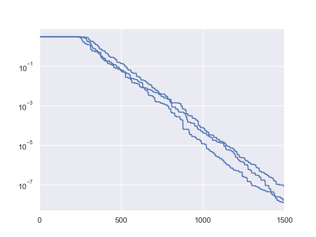
Below is a simple example to visualize the fitness convergence procedure of Evolution Strategy (ES) on the classical sphere function:

>>> import numpy as np  # https://link.springer.com/chapter/10.1007%2F978-3-662-43505-2_44
>>> import seaborn as sns
>>> import matplotlib.pyplot as plt
>>> from pypop7.benchmarks.base_functions import sphere
>>> from pypop7.optimizers.es.res import RES
>>> sns.set_theme(style='darkgrid')
>>> plt.figure()
>>> for i in range(3):
>>>     problem = {'fitness_function': sphere,
...                'ndim_problem': 10}
...     options = {'max_function_evaluations': 1500,
...                'seed_rng': i,
...                'saving_fitness': 1,
...                'x': np.ones((10,)),
...                'sigma': 1e-9,
...                'lr_sigma': 1.0/(1.0 + 10.0/3.0),
...                'is_restart': False}
...     res = RES(problem, options)
...     fitness = res.optimize()['fitness']
...     plt.plot(fitness[:, 0], np.sqrt(fitness[:, 1]), 'b')  # sqrt for distance
...     plt.xticks([0, 500, 1000, 1500])
...     plt.xlim([0, 1500])
...     plt.yticks([1e-9, 1e-6, 1e-3, 1e0])
...     plt.yscale('log')
>>> plt.show()

Algorithm Selection and Configuration

For most real-world BBO, typically there is few a prior knowledge to serve as the base of algorithm selection. Perhaps the simplest way to algorithm selection is trial-and-error. However, here we still hope to provide a rule of thumb to guide algorithm selection according to algorithm classification. Refer to its GitHub homepage for details about three different classification families (only based on the dimensionality). It is worthwhile noting that this classification is just a very rough estimation for algorithm selection. In practice, the algorithm selection should depend mainly on the final performance criteria ( e.g. convergence rate / solution quality / runtime).

In the future, we expect to add the Automated Algorithm Selection and Configuration techniques in this library, as shown below (just to name a few):

• Lindauer, M., Eggensperger, K., Feurer, M., Biedenkapp, A., Deng, D., Benjamins, C., Ruhkopf, T., Sass, R. and Hutter, F., 2022. SMAC3: A versatile Bayesian optimization package for hyperparameter optimization. Journal of Machine Learning Research, 23(54), pp.1-9.

• Schede, E., Brandt, J., Tornede, A., Wever, M., Bengs, V., Hüllermeier, E. and Tierney, K., 2022. A survey of methods for automated algorithm configuration. Journal of Artificial Intelligence Research, 75, pp.425-487.

• Kerschke, P., Hoos, H.H., Neumann, F. and Trautmann, H., 2019. Automated algorithm selection: Survey and perspectives. Evolutionary Computation, 27(1), pp.3-45.

• Hoos, H.H., Neumann, F. and Trautmann, H., 2017. Automated algorithm selection and configuration (Dagstuhl Seminar 16412). Dagstuhl Reports, 6(10), pp.33-74.